[ Meshtastic RF Coverage Planning ]

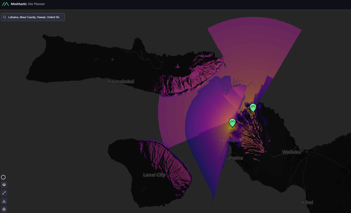
The Meshtastic Site Planner predicts where a Meshtastic node's signal will
actually reach — a terrain-aware RF coverage map you can read before climbing
a hill or buying an antenna. You drop a transmitter at a lat/lon, describe the
radio and antenna on both ends, set the propagation environment, and it renders
a heat-map of predicted received signal strength (RSSI in dBm) over the
surrounding terrain.

It's the Meshtastic-flavored cousin of tools like SPLAT!, Radio Mobile, and
CloudRF, with sensible LoRa defaults baked in. This guide walks every setting,
explains how the underlying model uses it, and ends with a worked example and
the one gotcha that quietly wrecks coastal/island plans.

Why bother? At 900 MHz, LoRa range is dominated by two things the
math can predict: antenna height and terrain line-of-sight. A node 8 m up on a
ridge can outrange a 30 m-tower node stuck behind a hill. The planner shows you
that before you commit hardware to a rooftop.

The planner uses the Longley-Rice Irregular Terrain Model (ITM)
— the same propagation model SPLAT! uses. It combines:

  — Terrain elevation sampled from a digital elevation
    model along every path from the transmitter, so hills, ridges, and valleys
    shadow the signal realistically.
  — Free-space + diffraction + tropospheric scatter loss
    for each path, based on distance and frequency.
  — Statistical fading margins (the situation / time
    fractions below) so the prediction is a confidence level, not a
    single deterministic number.

Everything you set in the config feeds those three. The output dBm at each map
pixel is then compared against your receiver sensitivity: above it = a link is
predicted, below it = no link.

The node doing the transmitting — location, radio, and antenna.

  tx_lat / tx_lon     Decimal degrees. Where the node sits. The
                       model samples terrain outward from here.
  tx_power            Conducted RF output in watts.
                       Meshtastic firmware sets this in dBm; convert:
                       dBm = 10 × log10(power_mW). e.g. 0.158 W = 158 mW
                       ≈ 22 dBm. Common US ceiling is
                       30 dBm (1 W) but most radios top out ~22-27 dBm.
  tx_freq             Center frequency in MHz.
                       Use your region's band: US 902-928 (e.g. 906-915),
                       EU 868, ANZ 915-928, etc. Frequency sets path loss
                       (higher = more loss) and must match your hardware region.
  tx_height           Antenna height in metres above
                       ground (AGL), NOT above sea level. The single
                       highest-leverage number in the whole config —
                       doubling height often beats doubling power.
  tx_gain             Antenna gain in dBi. A
                       stock whip is ~2-3 dBi; a high-gain colinear 5-8 dBi.
                       Gain trades vertical beamwidth for range — very
                       high gain on a hilltop can overshoot nearby valleys.

EIRP (effective radiated power) ≈ tx_power(dBm) + tx_gain(dBi) − cable
loss. The model radiates that.

The assumed node on the OTHER end — defines the threshold for "is there
a link here?" The map is drawn from this node's point of view.

  rx_sensitivity      The weakest signal (dBm) the receiver can
                       still decode. This is set by your LoRa preset
                       (spreading factor / bandwidth), not the chip alone.
                       Rough SX126x figures:
                         LongFast  (SF11/BW250)  ≈ −129 dBm
                         LongSlow  (SF12/BW125)  ≈ −134 dBm
                         MediumFast(SF9/BW250)   ≈ −124 dBm
                       Lower (more negative) = hears weaker signals = more range,
                       at the cost of airtime/throughput. −130 is a fair
                       LongFast-ish default.
  rx_height           Receiver antenna height AGL (m). 1 m models
                       a handheld; raise it for a fixed station.
  rx_gain             Receiver antenna gain (dBi).
  rx_loss             Feedline / connector loss (dB) on the RX side.

The link budget the map evaluates per pixel:
  received_dBm = EIRP − path_loss(terrain, freq, distance) + rx_gain − rx_loss
A pixel "has coverage" when received_dBm ≥ rx_sensitivity.

The propagation medium — these tune the Longley-Rice model. Defaults are
usually fine EXCEPT radio_climate near coastlines (see the gotcha below).

  radio_climate       Longley-Rice climate zone. Picks the
                       atmospheric statistics for your region:
                         equatorial, continental_subtropical,
                         maritime_subtropical, desert,
                         continental_temperate,
                         maritime_temperate_overland,
                         maritime_temperate_oversea
                       Get this right for islands/coasts —
                       see below.
  polarization        vertical or horizontal. Meshtastic whips are
                       vertical — leave it vertical unless
                       you've deliberately mounted antennas sideways.
  clutter_height      Ground clutter (trees/buildings) height in m
                       the signal must clear near each end. 1 m ≈ open;
                       raise for forest/urban to model the canopy/rooftop loss.
  ground_dielectric   Relative permittivity of the ground. 15 =
                       "average ground" (SPLAT! default). Sea water ≈ 80,
                       poor/dry ground ≈ 4-5.
  ground_conductivity Ground conductivity (S/m). 0.005 = average
                       ground; sea water ≈ 5.0; dry/rock ≈ 0.001.
                       Matters most for ground-wave at low VHF; minor at 900 MHz.
  atmosphere_bending  Surface refractivity in N-units. 301 =
                       standard atmosphere. Higher values model more
                       ducting/bending (over-water can exceed 350 and carry
                       signals far beyond line-of-sight).

How the prediction is computed — reliability, area, and resolution.

  situation_fraction  % of locations the prediction holds
                       for (Longley-Rice "location variability"). 95 = "the
                       signal is at least this strong at 95% of spots in each
                       pixel." Higher = more conservative (smaller, safer map).
  time_fraction       % of time the prediction holds
                       (fading over time). 95 = conservative. Planning a
                       reliable link? Keep both at 90-95. Want a best-case
                       "how far could it reach?" map? Drop to 50.
  simulation_extent   Radius in km to compute around the TX.
                       Bigger = slower. Size it to your realistic range
                       (LoRa rarely beats 30-50 km without exceptional height).
  high_resolution     false = faster, coarser terrain sampling
                       (good for a quick look). true = finer DEM sampling =
                       slower but catches narrow ridges, notches, and
                       fresnel-grazing terrain. Use true for a final plan in
                       hilly country.

Pure cosmetics — how the heat-map is drawn. No effect on the physics.

  color_scale          Palette (plasma, viridis, etc.). plasma
                       reads well on terrain imagery.
  min_dbm / max_dbm    The dBm range mapped across the color
                       ramp. Setting min_dbm to your rx_sensitivity makes the
                       map's edge = the actual link limit. max_dbm just sets
                       where the "very strong" end saturates.
  overlay_transparency % see-through of the overlay so the base
                       map/terrain shows through. 50 is a good balance.

A real config for a South-Maui node, decoded from a Site Planner share link.
This is the JSON the #cfg= URL fragment carries (base64-encoded):

transmitter:
  name: "Caloric Tuna"
  tx_lat: 20.957038        # South Maui (~Kihei)
  tx_lon: -156.683474
  tx_power: 0.158          # 158 mW  ~= 22 dBm
  tx_freq: 907             # US 915 ISM band
  tx_height: 8             # 8 m antenna AGL
  tx_gain: 3               # ~stock-to-modest whip
receiver:
  rx_sensitivity: -130     # LongFast-ish floor
  rx_height: 1             # handheld
  rx_gain: 2
  rx_loss: 2
environment:
  radio_climate: continental_temperate   # <-- see the gotcha below
  polarization: vertical
  clutter_height: 1
  ground_dielectric: 15    # average ground
  ground_conductivity: 0.005
  atmosphere_bending: 301  # standard atmosphere
simulation:
  situation_fraction: 95   # conservative / reliable
  time_fraction: 95
  simulation_extent: 30    # km radius
  high_resolution: false   # quick-look
display:
  color_scale: plasma
  min_dbm: -130
  max_dbm: -80
  overlay_transparency: 50

Reading it: a 22 dBm node, 8 m up, modest 3 dBi antenna,
into a handheld at the LongFast sensitivity floor, computed conservatively
(95/95) over a 30 km radius. A sensible "what can my hilltop node reliably
reach?" plan — with one setting wrong (next section).

The example above sets radio_climate: continental_temperate —
but the node is on Maui, a Pacific island. That's the most
common Site-Planner mistake for coastal and island operators.

Why it matters: the radio climate selects the atmospheric
statistics Longley-Rice uses for fading and over-horizon propagation. Over open
ocean, a maritime climate models the elevated refractivity and
ducting that routinely carry 900 MHz signals well past optical
line-of-sight — the exact mechanism behind those surprising island-to-island
Meshtastic contacts (Maui ↔ Lanaʻi / Molokaʻi / Kahoʻolawe).
A continental climate doesn't model that, so it tends to under-predict
your real over-water range.

Fix: for Hawaii (~21° N, subtropical and surrounded by sea):
  — maritime_subtropical is the closest single match.
  — maritime_temperate_oversea is the better pick if your
    important paths are mostly over water and you want the over-sea statistics.
Either beats continental_temperate for an island. Mainland-coastal
US nodes generally want maritime_temperate_overland/oversea.

It won't change line-of-sight terrain shadowing — that's elevation-driven
— but it meaningfully changes the predicted reach of the marginal,
over-water, beyond-horizon paths that island meshes live and die on.

  — Height beats power. Before adding watts or a bigger
    antenna, model +5 m of mast. It almost always wins, and it's legal
    everywhere.
  — Match rx_sensitivity to your actual preset. Planning
    a LongFast mesh but simulating at −134 (LongSlow) paints coverage you
    won't have. Set it to the preset you'll really run.
  — Two maps tell the story: run 95/95 for the "reliable
    everyday" footprint, then 50/50 for the "best-case DX" reach. The gap
    between them is your marginal zone.
  — Turn on high_resolution for the final plan in hilly
    terrain (all of Maui) — coarse sampling can miss a single ridge that
    makes or breaks a path.
  — Mind the law. tx_power + gain is EIRP; stay within
    your region's limit (US: generally 30 dBm conducted, with EIRP allowances).
    The planner won't stop you simulating an illegal config.
  — Validate in the field. The model is a prediction.
    Confirm with a real node and the Meshtastic app's signal readings, then
    tune your assumptions (clutter_height especially) to match reality.

Steep volcanic terrain is the hardest case — deep amphitheater valleys,
knife-edge ridges, and dense wet canopy all fight you at once. Mauna Kahalawai
(the West Maui Mountains) is the textbook example: 1,700 m+ ridges, valleys like
ʻĪao / Waiheʻe / Olowalu / Ukumehame walled off on three sides, and a summit
zone near Puʻu Kukui that's among the wettest places on Earth. Tips that
actually move the needle there:

  — Think mesh topology, not a coverage circle. No single
    node blankets a massif — nothing will. Meshtastic is multi-hop: put
    fixed router/repeater nodes on ridgelines and saddles so each one
    owns a valley or two and relays to the next. Use the planner per-candidate-
    site to choose each relay's ridge, not to chase one giant footprint.

  — Go AROUND the mountain, not over it. A coastal chain
    (Lahaina → Kāʻanapali → Kapalua → Kahakuloa) links via
    over-water paths that routinely beat trying to punch over a 5,000 ft ridge.
    This is exactly why radio_climate should be
    maritime_* here — model those coastal hops with the
    over-sea statistics.

  — Exploit saddles and passes as RF "windows." Signal
    can't pass through a ridge, but it squeezes through the low gaps between
    peaks. Find the saddles (e.g. toward the central isthmus / Kahului) and aim
    nodes to shoot through them into otherwise-shadowed valleys. Place the TX
    where a saddle gives it line-of-sight into the target.

  — Model from the valley's point of view, in high-res.
    Turn high_resolution ON — coarse sampling misses the one
    ridge notch that makes or breaks a link. For a specific target (a node in
    ʻĪao Valley, say), put the receiver in the valley and the
    transmitter on the candidate ridge; the diffraction over the valley rim is
    where the link budget lives or dies.

  — Budget for canopy and rain. The wet windward slopes
    carry dense, saturated vegetation; at 915 MHz that's real, persistent loss
    (easily 10-20+ dB through deep wet canopy). Raise clutter_height
    to model the canopy near valley-floor nodes and don't plan to the bare-
    terrain best case.

  — Directional antennas on valley-feed relays. A ridge
    node with an omni wastes most of its power skyward and out to sea. A yagi or
    panel aimed down into the target valley concentrates gain where you need it
    — model it by raising tx_gain and noting the aim heading.
    Trade-off: a directional only serves what it points at, so it's for
    dedicated valley feeds, not general mesh nodes.

  — Height clears the Fresnel zone, not just line-of-sight.
    A path that grazes a ridge top still loses signal because terrain intrudes
    into the Fresnel zone. On knife-edge ridges, a few extra metres of mast to
    clear the obstruction by a real margin pays off more than it would on flat
    ground — another case of height beating power.

  — Power you can sustain beats coverage you can't. The
    summit zone is cloud-wrapped and soaked most of the year, so solar is
    unreliable up high. A reachable, sunnier lower ridge or coastal high point
    often makes a better permanent relay than the true peak, even when
    the peak models better. Validate every candidate in the field — on
    this kind of terrain the model is a starting hypothesis, not gospel.

The Site Planner encodes the entire config into the URL after
#cfg= as base64-encoded JSON. That means:

  — A share link is self-contained — no account, no
    server-side save. Anyone who opens it sees your exact plan.
  — You can decode/inspect one yourself: base64-decode the
    part after #cfg= to get the JSON (that's how the worked example
    above was recovered).
  — It's also diff-able and version-able — drop the
    decoded JSON in a repo to track changes to a site plan over time.

Decode one from a shell:

# everything after '#cfg=' is base64-encoded JSON
echo '<cfg-string>' | base64 -d | python3 -m json.tool